


Predicting the Market with Machine Learning
A simple cross-sectional, self-filtering approach.

Before we get started, I’d like to thank Marcos López de Prado and his book Advances in Financial Machine Learning. His work has helped me significantly when it comes to understanding how machine learning connect with trading as well as some of the flaws that might be encountered while testing.
If you are interested in learning how to apply machine learning yourself then I would definitely recommend checking out his work. I’ll include a link below for his book.
In this paper, I will discuss two novel approaches for applying machine learning to stock price prediction. Three models are tested as well as an ensemble method using a voting regressor.
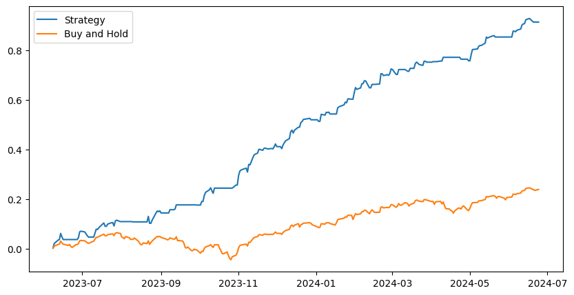
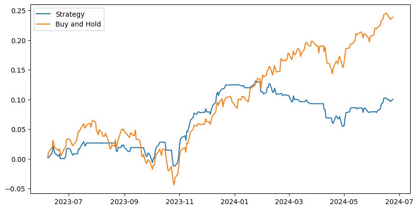
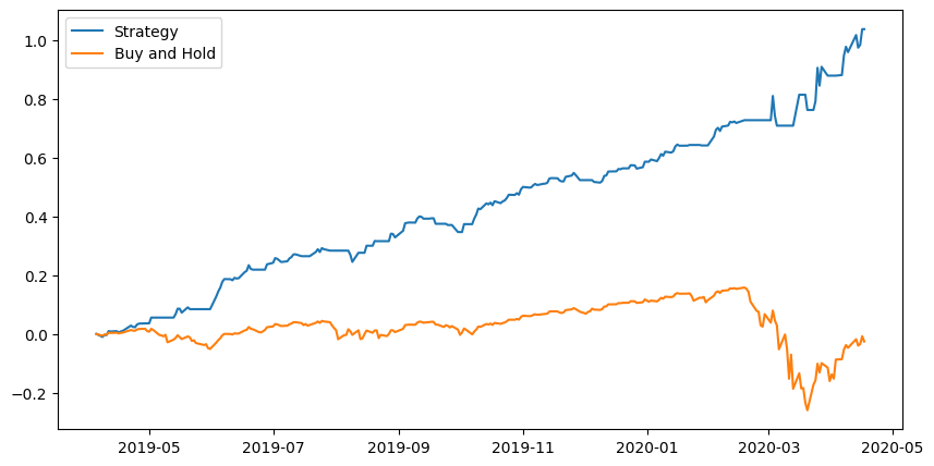
The results show the model’s ability to handle market downturns and capture upside in the process. The model outperforms buy and hold by a good margin.
Here is what the performance looks like:
If you are interested in learning more about this methodology or looking to trade the model then join our discord server using the button below.
History
Machine learning and AI are not new concepts when it comes to predicting the stock market. In fact, researchers started looking into this just years after the first commercially avaliable computers.

In 1987, Braun and Chandler published a paper titled, "Predicting Stock Market Behavior Through Rule Induction: An Application of the Learning-From-Example Approach." At the time, the newest computers had 4KB of memory as opposed to the recommended minimum of 4GB these days… and that’s not even considering the differences in other technological advancements in computer memory.
Needless to say, predicting the future of the stock market is a mystery that is yet to be solved.
New Approach
In this paper, I will present two new approaches to financial machine learning. An inspiration for these was presented in Advances in Financial Machine Learning
Price series are often non-stationary, and often have memory. In contract, integer differentiated series, like returns, often have a memory cut-off, in the sense that history is disregarded entirely after a finite sample window.
- López de Prado, 2018, p. 75
What López de Prado discussed in this chapter is that it is important to preserve ‘memory’ of prices. For example, an RSI value of 30 after a severe market downturn is different than an RSI value of 30 after a small pullback in a bull market. Machine learning models require a discrete sample to learn from so the challenge becomes integrating the most amount of information about the past into just 1 data point.
Methodology
Since we are trying to predict the broad market, we need to be broad in our feature selection as well.
Simply passing in data from SPY will be unlikely to yield significant results due to multitude of external variables. For example, there are various factors which could cause SPY to drift from its fair value as per the SPX — how is the model supposed to interpret these events when it is being trained to understand trend?
To gather basic features, we’ll get daily price data from each sector within the S&P 500. We will also get the VIX and some macroeconomic indicators.
These alone, will be unlikely to yield results due to the non-stationary of the prices — using x-period of returns would make the data stationary but remove memory.
Instead, we will use slope and convexity of price to capture the dynamic over a fixed lookback window. Of course, it would be ideal if we could consider all the data but this is very difficult to capture in just one indicator.
By measure slope and convexity of price over various windows we get an idea of the parametric curve which should ideally retain a decent amount of memory regarding momentum patterns, top/bottom price formations, and various other significant events.
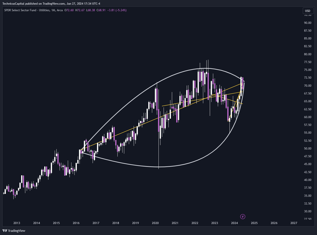
Below is an example of measuring slope and convexity. The yellow lines indicate the slope over a given period of time, while the white curves indicate convexity and concavity of price. These show to be very strong predictive features.
Training the Model
With our freshly processed dataset we can begin training our model. A classic approach is to attempt at predicting the forward x-day return. However, once again this retains no memory. Another issue with this, as mentioned by López de Prado is that forecasting forward returns does not account for any price volatility within the period. This is unrealistic and could lead to increased portfolio volatility.
Instead, we will predict the bisecting forward slope of the price.
In theory, if we can predict this bisecting slope going forward a few days. Then we should be able to stay long during uptrends and go flat or even short during downtrends.
K-Nearest Neighbors
A simple and interpretable approach is the KNN Algorithm. This is a supervised learning model in which historical samples with similar feature values are allowed to cast a vote on what they think the outcome will be. There are many ways to tune this model such as: distance metric, size of K, weighted voting, etc.
For this study, we used 7 neighbors and the Lorentzian distance metric.
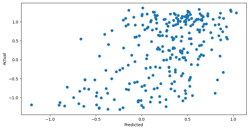
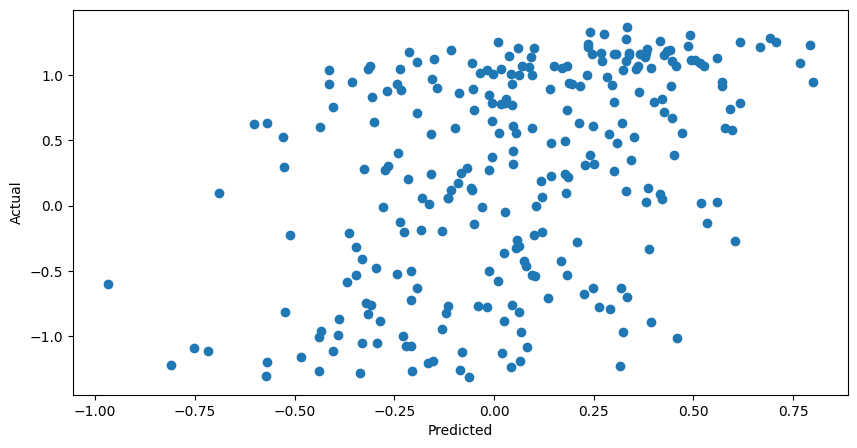
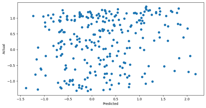
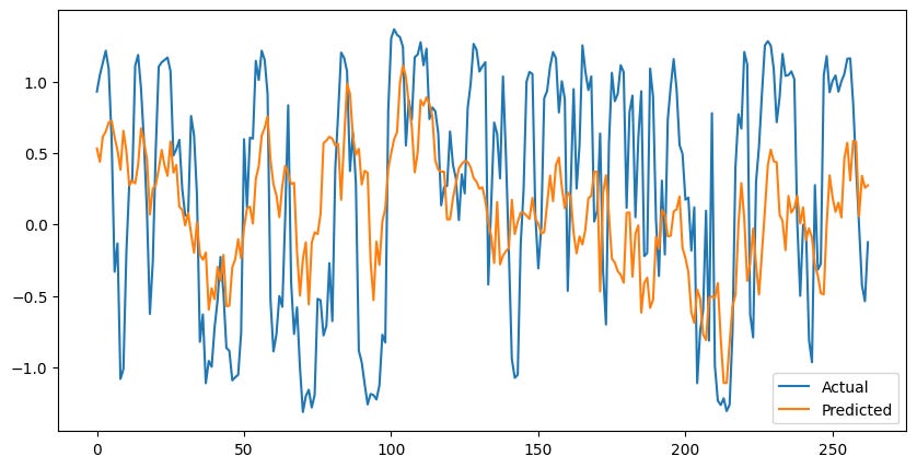
Nice! The model is finding some kind of relationship and has a moderate, positive correlation when predicting the actual values.
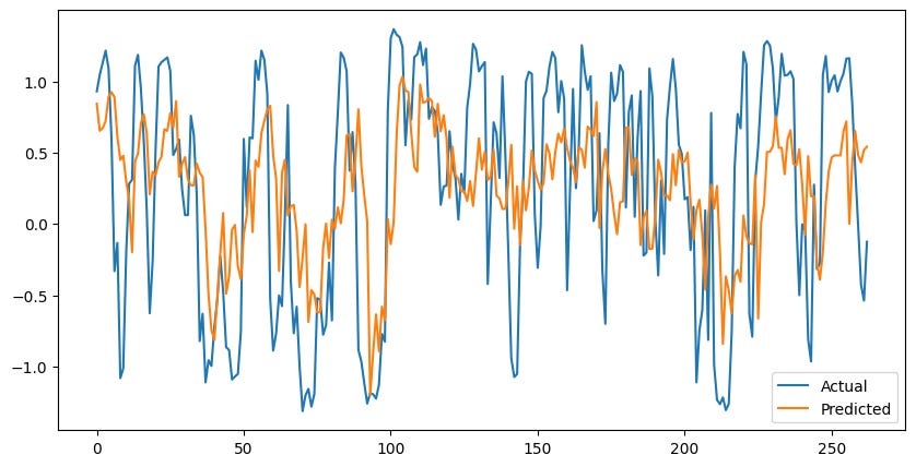
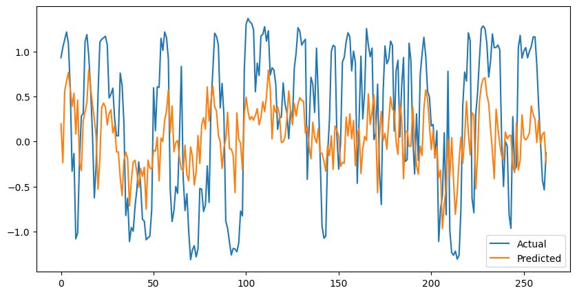
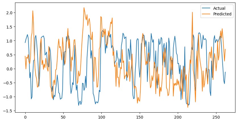
This model can respond quickly to changes and gets relatively close to the actual values.
Unfortunately, at times this model can lag behind and be exposed to some downturns or miss upside
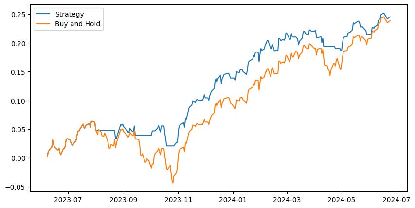
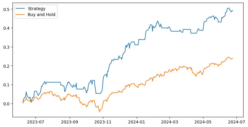
Without any filters, the model is able to match the performance of the S&P500 while reducing volatility. Let’s give it some leverage.
Further outperformance with less volatility… I like it. With nearly 30% excess returns we should easily be able to cover margin costs — especially since we don’t have 100% exposure.
Extreme Gradient Boosting
XGBoost is pretty much just an overcomplicated decision tree. It works by splitting the data into samples and training decision trees for each (boosting).

Let’s run XGBoost and see how it performs with our data.
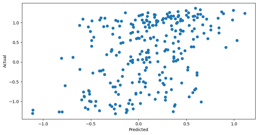
Interestingly, the model has a similar pattern between its predictions and the actual values. It seems as though both of these models are using historical references which might not account for extreme values.
However, the XGBoost seems to adjust to, and even predict future values of the future… Weird?
The model underperformed buy and hold. However, we will still save this for later when we test a voting regressor pipeline.
Multi-Layer Perceptron Network
Now its time for the fun stuff… I hope. Maybe the relationship we are looking for is not actually linear but more complex.
Let’s bring out the big guns and run an unsupervised learning model. Maybe this neural network can see something that we can’t.
Nevermind… While the model is able to synchronize with reality on some occasions. It performed the worst in terms of error.
Ensemble Method Using a Voting Regressor
Throwing around fancy words is fun, but in reality this is pretty simple. Allow all the models to forecast and cast their vote, then take the average or some weighted average and use that as the prediction.
A slight improvement.
A Novel Filtering Approach
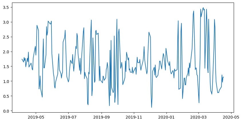
Now, all of these charts got me thinking and one thing that I noticed was the models inability to handle severe and extended downturns. These models can respond well to high positive values, but begin to show high error with low values.
I would guess that this is due to the lack of samples from bearish markets. However, another pattern I noticed is that the model can quickly adjust and synchronize, but when it loses synchronicity then it often stays unsynchronized for some time before correcting itself.
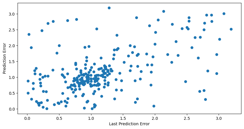
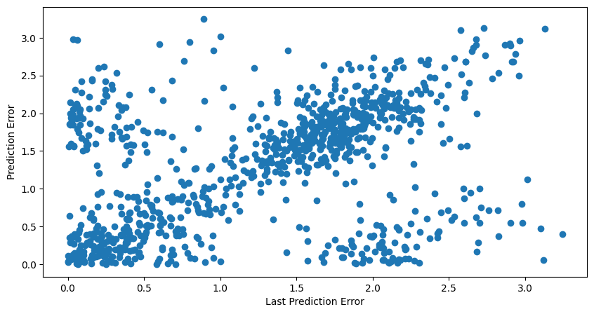
Below is chart comparing the previous prediction error vs the next prediction error.
We see that high values of prediction error are correlated with high values of future prediction error. Once again, likely during bear markets where the model has insufficient samples to make a good prediction.
Is this a problem? Maybe not, do we really need to be invested during bearish markets?
Let’s filter our trades and avoid trading if the prediction error from last prediction was high. This has to be fine-tuned depending on the specific model since all will yield various error thresholds.
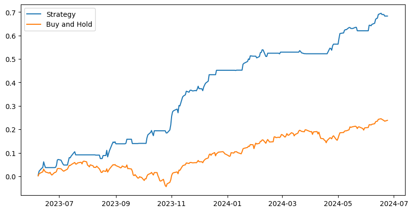
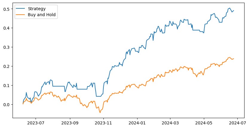
And here it is! The system holds a long position when the predicted bisecting slope is positive and the previous days error was below the 80th percentile.
It returned 70% over the past year with almost no volatility. The margin aspect is very important here because the system has relatively low market exposure and needs a boost to compensate for some missed rallies.
Stress Testing
Once again, borrowing an idea from king Marcos to test and see how the model would have performed during various historical scenarios that might have wiped it out.
For the following tests, the train/test data will be adjusted to include the desired scenario within the testing sample. The model will have no knowledge of the scenario that we are testing.
Testing the COVID crash
Great results, and you can see how the model error spikes right around the times when the market starts to pull back. Unusual model predictions began occurring right at the top, days before the COVID crash began. My guess would be that it expected a change in trend down a few days before it actually occurred and the price kept rallying contrary to what typically occurs.
Testing the 2008 Financial Crisis
In order to perform this test, I had to remove two sector ETF’s that did not have data during that time. This allowed the model to train on much more data — three times as much. Let’s see what happened.
The prediction error filter has even more significance with the higher magnitude of data we have given it.
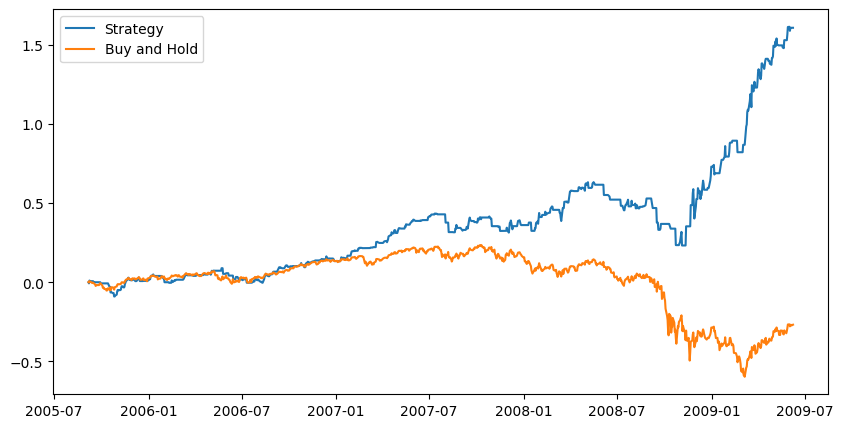
So you can profit during a bear market, huh.
Remember this model is long-only… It does not short! Very impressive results.
Conclusion
That was a lot of content. To sum it up, we tested 3 different machine learning models, supervised and unsupervised. We also tested a voting classifier as an ensemble method.
By creating informative features that can retain market memory as well as choosing a stationary target variable which also has some memory of its own; we can train machine learning models to identify the future slope in price and subsequently profit from any moves to the upside.
Our results are consistent with the saying, “Keep it simple, stupid!”. The simple KNN model performed extremely well compared to the others including the ensemble method.
We also presented a novel approach for time series forecasting, which takes advantage of the autocorrelation properties of financial assets. Using the previous prediction error as a filter works very well in our testing and allows for avoiding areas of uncertainty — which are usually associated with downward moves in the market.
The Best Part… It’s free!
We will be posting daily predictions in our discord group for free — not forever. If you are interested in discussing machine learning, quant finance or even just general trading then join the discord to find a group of like-minded researchers.
Amazing work done here!